AMFusionCore

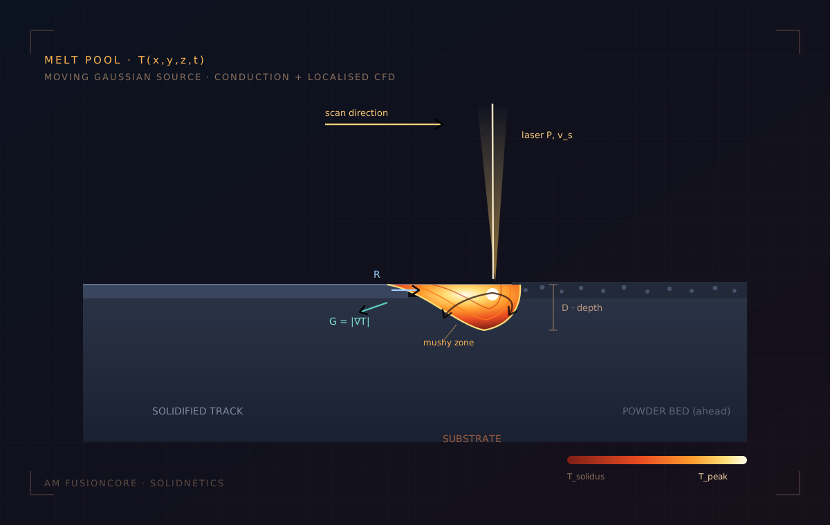
Where PathWeaver is pure geometry, FusionCore is pure physics: transient heat transfer with phase change, a moving Gaussian source, and localised CFD wherever the metal is molten. The most expensive solver in the stack — and the one that resolves what actually happens to the material.

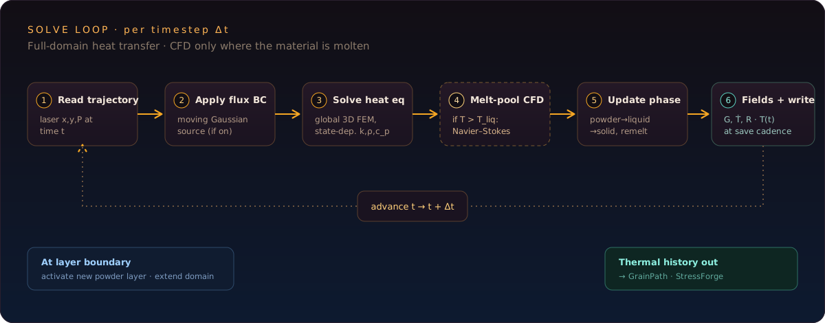
The solver advances one timestep at a time. The heat equation is solved across the full domain on every step; the CFD step runs only where T > T_liquidus — a small subdomain that travels with the laser. New powder layers are activated as the build grows upward.

FIG.01 · fusioncore_solve_loop full-domain heat transfer · CFD only where molten

Six features that define what FusionCore resolves at every timestep.

Transient heat transfer with phase change

Full 3D conduction with state-dependent thermal properties — every node tracked from powder to solid:

• State-dependent k, ρ, c_p (per phase, temperature-dependent)
• Apparent-heat-capacity treatment of latent heat L_f
• Mushy-zone resolution across T_solidus → T_liquidus
• Powder → liquid → solid transitions, including remelting

Moving Gaussian laser model

The laser is a moving flux boundary condition — driven directly by the trajectory's per-segment schedule:

• Gaussian intensity profile with configurable spot size
• Absorptivity coefficient per material (or T-dependent)
• Power & scan-speed sourced from trajectory.json
• Galvo jump moves preserved — laser off during repositioning
• Multi-laser ready: each laser_id applied as an independent source

q(x, y, t) = 2 η P / (π r₀²)
            · exp(−2 r²/r₀²)

η  · absorptivity
P  · laser power [W]
r₀ · 1/e² spot radius [m]
r  · distance to beam centre

Localised melt-pool CFD

When and where the metal is molten, FusionCore engages a full Navier–Stokes solve — but only there:

• Marangoni-driven recirculation from surface-tension gradients
• Buoyancy & thermocapillary coupling
• Resolves melt-pool width, depth, length per timestep
• Optional keyhole physics for deep-penetration regimes
• Skips automatically wherever T < T_liquidus

Width W

120–180 µm
typical LPBF

Depth D

60–120 µm
conduction mode

Length L

300–600 µm
scan-speed dependent

CFD region

~0.1 %
of full domain

Solidification fields (G, Ṫ, R)

FusionCore writes the three per-node fields that define solidification behaviour:

• G = |∇T| — thermal gradient at the solidification front
• Ṫ = ∂T/∂t — cooling rate through the mushy zone
• R = v_n — solidification velocity normal to the front

These fields feed GrainPath's columnar-to-equiaxed transition map and microstructure prediction directly.

node 14201
  T_peak  = 2 184 K
  G       = 1.8e7 K/m
  Ṫ       = 4.2e6 K/s
  R       = 0.62 m/s
  state   = solid
  remelts = 2 → 1

Three fidelity modes

Pick resolution against the compute budget. Every mode reads the same trajectory and writes the same field schema — only the spatial extent and mesh resolution change.

Melt-pool

Single-track

Resolve melt-pool geometry, Marangoni flow, and keyhole physics on millimetre tracks.

~10 µm mesh · minutes

Part scale

Full-part

Whole-build thermal history with adaptive coarsening below the active layer.

~200 µm mesh · days

Validated materials & solver stack

FusionCore ships with validated material cards for the four canonical LPBF alloys, with temperature-dependent properties through liquidus:

SS316L Ti-6Al-4V IN718 AlSi10Mg

Custom materials added through the Material Library — define k(T), ρ(T), c_p(T), T_sol, T_liq, L_f.

FEniCSx · FEM DOLFINx · CFD Gmsh · mesh

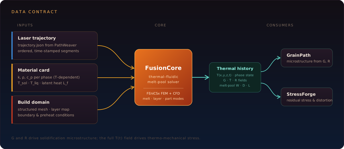
FusionCore sits between geometry and prediction. Its single thermal-history output is the shared currency of the back half of the stack — GrainPath reads G and R for microstructure, StressForge reads the full T(t) field for residual stress.

FIG.02 · fusioncore_io_contract trajectory + material + domain → T(x,y,z,t) · G · Ṫ · R

FusionCore consumes PathWeaver's trajectory and produces the thermal history that splits into the two downstream prediction paths — microstructure (GrainPath) and stress (StressForge).

A full-part LPBF thermal solve can need hundreds of CPU-hours. SolidNetics elastically schedules those across cloud workers so you press Run and walk away.

Three steps from a trajectory file to a complete thermal record of the build.

Built for LPBF process engineers tuning parameter windows, machine builders validating new heads and lasers, and research teams investigating melt-pool physics, microstructure, and defect formation.